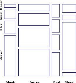
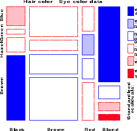
Figure 17: Condensed mosaic for Hair-color, Eye-color data. Each column is divided according to the conditional frequency of eye color given hair color. The area of each rectangle is proportional to observed frequency in that cell.
In the column proportion mosaic , the width of each box is proportional to the total frequency in each column of the table. The height of each box is proportional to the cell frequency, and the dotted line in each row shows the expected frequencies under independence. Thus the deviations from independence, f sub ij - e sub ij , are shown by the areas between the rectangles and the dotted lines for each cell.
The amount of empty space inside the mosaic plot may make it
harder to see patterns, especially when there are large deviations
from independence. In these cases, it is more useful to separate the
rectangles in each column by a small constant space, rather than
forcing them to align in each row. This is done in the
condensed mosaic display Again, the area of each box is
proportional to the cell frequency, and complete independence is
shown when the tiles in each row all have the same height.
Figure 17: Condensed mosaic for Hair-color,
Eye-color data. Each column is divided according to the conditional
frequency of eye color given hair color. The area of each rectangle
is proportional to observed frequency in that cell.
In Hartigan & Kleiner's (1981) original version, all the tiles are unshaded and drawn in one color, so only the relative sizes of the rectangles indicate deviations from independence. We can increase the visual impact of the mosaic by:
The condensed form of the mosaic plot generalizes readily to the display of multi-dimensional contingency tables. Imagine that each cell of the two-way table for hair and eye color is further classified by one or more additional variables--sex and level of education, for example. Then each rectangle can be subdivided horizontally to show the proportion of males and females in that cell, and each of those horizontal portions can be subdivided vertically to show the proportions of people at each educational level in the hair-eye-sex group.
for all i , j , k in a three-way table. This corresponds to the log-linear model [A] [B] [C] . Fitting this model puts all higher terms, and hence all association among the variables into the residuals.(6)
This corresponds to the log-linear model is [ A B ] [ C ] . Residuals from this model show the extent to which variable C is related to the combinations of variables A and B but they do not show any association between A and B .(7)
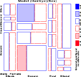
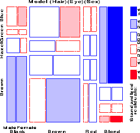
Figure 20: Mosaic display for hair color,
eye color, and sex. This display shows residuals from the model of
complete independence, [H] [E] [S], G² = 179.79 on 24 df.
For a three-way table, the the hypothesis of complete independence, H sub { A otimes B otimes C } can be expressed as
where H sub { A otimes B } denotes the hypothesis that A and B are independent in the marginal subtable formed by collapsing over variable C , and H sub { AB otimes C } denotes the hypothesis of joint independence of C from the AB combinations. When expected frequencies under each hypothesis are estimated by maximum likelihood, the likelihood ratio G ² s are additive:(8)
For example, for the hair-eye data, the mosaic displays for the {Hair} {Eye} marginal table and the [HairEye] [Sex] table can be viewed as representing the partition(9)
Model                      df        G²

{Hair} {Eye}                9       146.44
[Hair, Eye] [Sex]          15        19.86
------------------------------------------
[Hair] [Eye] [Sex]         24       155.20
This partitioning scheme extends readily to higher-way tables.