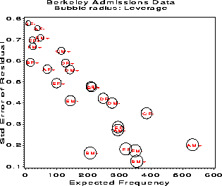
Figure 39: Standard errors of residuals decrease with expected frequency. This plot shows why ordinary Pearson and deviance residuals may be misleading.
Formally, however, log-linear models are closely related to ANOVA models for quantitative data. For two variables, A and B, for example, the hypothesis of independence means that the expected frequencies, m sub ij obey
m sub ij = < m sub i+ %% m sub +j > over m sub ++This multiplicative model can be transformed to an additive (linear) model by taking logarithms of both sides:
log ( m sub ij ) = log ( m sub i+ ) + log ( m sub +j ) - log ( m sub ++ )which is usually expressed in an equivalent form in terms of model parameters,
log ( m sub ij ) = mu + lambda sub i sup A + lambda sub j sup B (24)where mu is a function of the total sample size, lambda sub i sup A is the "main effect" for variable A, and lambda sub j sup B is the "main effect" for variable B, and the same analysis of variance restrictions are applied to the parameters: Sigma sub i %% lambda sub i sup A = Sigma sub j %% lambda sub j sup B = 0 . The main effects in log-linear models pertain to differences among the marginal probabilities of a variable. Except for differences in notation, the model (24) is formally identical to the ANOVA main-effects model for a two-factor design:
E ( y sub ij ) = mu + alpha sub i + beta sub jFor a two-way table, a model which allows an association between the variables is (the saturated model):
log ( m sub ij ) = mu + lambda sub i sup A + lambda sub j sup B + lambda sub ij sup AB (25)which is similar to the two-factor ANOVA model with interaction:
E ( y sub ij ) = mu + alpha sub i + beta sub j + ( alpha beta ) sub ijHence, associations between variables in log-linear models are analogous to interactions in ANOVA models. For example, in the Berkeley admissions data, the model
log % m sub ijk = mu + lambda sub i sup A + lambda sub j sup D + lambda sub k sup G + lambda sub ij sup AD + lambda sub ik sup AG + lambda sub jk sup DG (26)includes effects for associations between
log ( m sub < Admit (ij) > / m sub < Reject(ij) > ) = alpha + beta sub i sup Dept + beta sub j sup Gender (27)
To illustrate the reasoning here, consider the log-linear model
log % m sub ijk = mu + lambda sub i sup Sex + lambda sub j sup Treat + lambda sub k sup Outcome + lambda sub ij sup SexTreat + lambda sub ik sup SexOutcome + lambda sub jk sup TreatOutcome. (28)(or [SexTreat] [SexOutcome] [TreatOutcome], or [ST] [SO] [TO] in abbreviated notation) which was fit to test whether the association between treatment and outcome in the arthritis data was homogeneous across sex. This model includes the main effect of each variable and all two-way associations, but not the three-way association of sex * treat * outcome. The three-way term [STO] therefore forms the residual for this model, which is tested by the likelihood ratio G sup 2 below.
+-------------------------------------------------------------------+
|                                                                   |
|                  No 3-way association                             |
|     MAXIMUM-LIKELIHOOD ANALYSIS-OF-VARIANCE TABLE                 |
|                                                                   |
|   Source                   DF   Chi-Square      Prob              |
|   --------------------------------------------------              |
|   SEX                       1        14.13    0.0002              |
|   TREAT                     1         1.32    0.2512              |
|   SEX*TREAT                 1         2.93    0.0871              |
|   IMPROVE                   2        13.61    0.0011              |
|   SEX*IMPROVE               2         6.51    0.0386              |
|   TREAT*IMPROVE             2        13.36    0.0013              |
|                                                                   |
|   LIKELIHOOD RATIO          2         1.70    0.4267              |
|                                                                   |
+-------------------------------------------------------------------+
Because the likelihood ratio G sup 2 = 1.70 is not significant I can conclude this is an acceptable model. However, it may not be necessary to include all the remaining terms in the model, and the small chi² values for the terms [ST] and [SO] suggested that I might refit a reduced model excluding them.
G sup 2 = 2 %% Sum % n % log sub e ( n / m hat )is more commonly used, since it is the statistic that is minimized in maximum likelihood estimation.
The chi-square statistics printed for the individual terms in a log-linear model are based on Wald tests , a general methodology for testing whether a subset of the parameters in a model are zero. Wald tests are analogous to the Type III (partial) tests used in ANOVA and regression models. They test they hypothesis that the given terms can be deleted from the model, given that all other terms are retained.
With SAS, log-linear models can be fit using PROC CATMOD, a very general procedure for categorical modelling. Loglinear models can also be fit with PROC GENMOD (as of SAS 6.08), a new procedure for generalized linear models. In SAS/INSIGHT, the Fit (Y X) menu also fits generalized linear models. When one variable is a binary response, you can also fit the equivalent logit model with PROC LOGISTIC.
title 'Berkeley Admissions data';
proc format;
   value admit 1="Admitted" 0="Rejected"          ;
   value yn    1="+"        0="-"                 ;
   value dept  1="A" 2="B" 3="C" 4="D" 5="E" 6="F";
data berkeley;
   do dept = 1 to 6;
      do gender = 'M', 'F';
         do admit = 1, 0;
            input freq @@;
            output;
   end; end; end;
/* Admit  Rej  Admit Rej */
cards;
     512  313    89   19
     353  207    17    8
     120  205   202  391
     138  279   131  244
      53  138    94  299
      22  351    24  317
;
For log-linear models, the MODEL statement should specify
_RESPONSE_ to the right of the = sign; use
the LOGLIN statement to specify the model to be fit. When
the data are in frequency form, as here, use a WEIGHT
statement to specify the frequency variable.
proc catmod order=data
            data=berkeley;
   format dept dept. admit admit.;
   weight freq;
   model dept*gender*admit=_response_ /
         ml nogls
         noiter noresponse nodesign noprofile
         pred=freq ;
   loglin admit|dept|gender @2 / title='Model (AD,AG,DG)';
 run;
On the loglin statement, the "bar" notation
admit|dept|gender @2 means all terms up to two-way associations.
The printed output includes the following, which indicates that only the two-way terms DEPT*ADMIT and DEPT*GENDER are significant. In particular, there is no association between Gender and Admission.
+-------------------------------------------------------------------+
|                                                                   |
|                         Model (AD,AG,DG)                          |
|          MAXIMUM-LIKELIHOOD ANALYSIS-OF-VARIANCE TABLE            |
|                                                                   |
|        Source                   DF   Chi-Square      Prob         |
|        --------------------------------------------------         |
|        ADMIT                     1       262.45    0.0000         |
|        DEPT                      5       276.37    0.0000         |
|        DEPT*ADMIT                5       534.71    0.0000         |
|        GENDER                    1       197.99    0.0000         |
|        GENDER*ADMIT              1         1.53    0.2167         |
|        DEPT*GENDER               5       731.62    0.0000         |
|                                                                   |
|        LIKELIHOOD RATIO          5        20.20    0.0011         |
|                                                                   |
+-------------------------------------------------------------------+
Consequently, we drop the [AG] term and fit the reduced model (AD, % DG) . The RESPONSE statement produces an output dataset containing observed and predicted frequencies, used in the following section.
   response / out=predict;
   loglin admit|dept dept|gender / title='Model (AD,DG)';
 run;
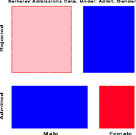
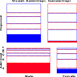
The overall fit of the model, shown by the likelihood-ratio G sup 2 = 21.7 on 6 df is not good. This, however, turns out to be due to the data for one department, as we can see in the mosaic display below.
We continue with the results from model (AD, DG) . Fitting the regression model for the working response using PROC REG is conceptually simple, though tedious because PROC REG (like PROC LOGISTIC) cannot generate the dummy variables itself. This must be done in a data step. In the PREDICT dataset, m hat sub i is named _pred_, n sub i is _obs_, and e sub i = n sub i - m hat sub i is _resid_.
data regdat;
   set predict;
   drop _sample_ _type_ _number_ i;
   where (_type_='FREQ');
   cell = trim(put(dept,dept.)) ||
          gender ||
          trim(put(admit,yn.));

   *-- Working response;
   y = log(_pred_) + _resid_/_pred_;

   *-- Construct dummy variables for the regression;
   array d{5}  d1-d5;
   array ad{5} ad1-ad5;
   array gd{5} gd1-gd5;
   g = (gender='M') - (gender='F');
   a = (admit=1) - (admit=0);
   do i=1 to 5;
      d(i)=(dept=i) - (dept=6);
      ad(i) = d(i) * a;
      gd(i) = d(i) * g;
      end;
The weighted regression of the working response is then performed
using the dummy variables as shown below. The output dataset is then
processed to multiply the Cook's D and studentized residual by the
appropriate factors of the MSE.
title2 'Diagnostics by weighted regression';
proc reg data=regdat outest=est;
   id cell;
   weight _pred_;
   model y = a g d1-d5 ad1-ad5 gd1-gd5;
   output out=regdiag
          h=hat cookd=cookd student=studres;
data regdiag;
   set regdiag;
   retain _rmse_;
   if _n_=1 then set est(keep=_rmse_ );
   adjres = studres * _rmse_;
   cookd = cookd * _rmse_**2;
The REGDIAG dataset is shown below. Note that all residuals are small in magnitude, except for those associated with Dept. A.
 CELL   _OBS_    _PRED_   _RESID_    COOKD      HAT     ADJRES

 AM+     512    531.431   -19.431    22.304    0.9588   -4.153
 AM-     313    293.569    19.431    11.892    0.9254    4.153
 AF+      89     69.569    19.431     2.087    0.6853    4.153
 AF-      19     38.431   -19.431     0.724    0.4304   -4.153
 BM+     353    354.188    -1.188     0.883    0.9842   -0.504
 BM-     207    205.812     1.188     0.507    0.9729    0.504
 BF+      17     15.812     1.188     0.026    0.6481    0.504
 BF-       8      9.188    -1.188     0.009    0.3945   -0.504
 CM+     120    113.998     6.002     0.058    0.5806    0.868
 CM-     205    211.002    -6.002     0.142    0.7734   -0.868
 CF+     202    208.002    -6.002     0.140    0.7701   -0.868
 CF-     391    384.998     6.002     0.295    0.8758    0.868
 DM+     138    141.633    -3.633     0.036    0.6873   -0.546
 DM-     279    275.367     3.633     0.086    0.8391    0.546
 DF+     131    127.367     3.633     0.031    0.6523    0.546
 DF-     244    247.633    -3.633     0.076    0.8211   -0.546
 EM+      53     48.077     4.923     0.054    0.4964    1.000
 EM-     138    142.923    -4.923     0.272    0.8306   -1.000
 EF+      94     98.923    -4.923     0.171    0.7552   -1.000
 EF-     299    294.077     4.923     0.619    0.9176    1.000
 FM+      22     24.031    -2.031     0.026    0.5531   -0.620
 FM-     351    348.969     2.031     0.672    0.9692    0.620
 FF+      24     21.969     2.031     0.022    0.5112    0.620
 FF-     317    319.031    -2.031     0.612    0.9663   -0.620
An influence plot can now be constructed by plotting the adjusted residual against leverage, using the value of Cook's D as the size of the bubble symbol at each point.
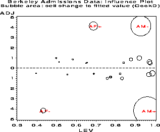

Figure 39: Standard errors of residuals
decrease with expected frequency. This plot shows why ordinary
Pearson and deviance residuals may be misleading.